Machine learning by itself sometimes isn’t the best answer, but it can be combined with specialist agents to expand it’s capabilities and reduce the training time. In the other hand, for simple problems, and specially for linear problems, usually machine learning can be replaced with more simple and precise approaches like linear programming.
Machine learning is the field of study that explores the construction of algorithms that learn from data and can make predictions about it. It is a field of artificial intelligence that uses statistical methods to give those predictions. And it’s name comes from the ability that it gives to computer systems to learn from data, without being explicitly programmed.
Since machine learning is strongly related to how you analyse your data, is the natural flow to learn first how to analyse your data, and then how to create your prediction models.
In statistics, regression analysis is the set of processes to estimate the relationship among variables.
Linear regression
In statistics, linear regression is a linear approach to modelling the relationship between a dependent variable and one or more independent variables. The dependent variable sometimes is referred as a scalar and the independent variables referred as explanatory variables.
Let’s use an example and explore it to make things easier to understand:
Given this set of variables
x = [10,8,13,9,11,14,6,4,12,7,5]
y = [8.04,6.95,7.58,8.81,8.33,9.96,7.24,4.26,10.84,4.82,5.68]
As raw data is hard to read and understand it, and if you count, the array has only 11 elements. In the real world your data will easily be far bigger than that.
We start our analysis by plotting our data to analyse its dispersion.
import numpy as np
import matplotlib.pyplot as plt

x = [10,8,13,9,11,14,6,4,12,7,5]
y = [8.04,6.95,7.58,8.81,8.33,9.96,7.24,4.26,10.84,4.82,5.68]

plt.scatter(x, y)
plt.show()
You should receive a image just like this
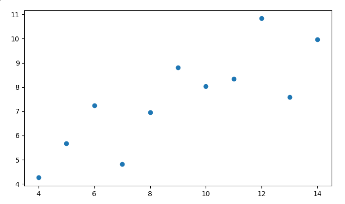
A simple look at it and you can determine that the \(Y\) value increases when the \(X\) value increases, there is a correlation, which we determined empirically, but for calculating our linear regression we have to formalize it, so this is when Pearson correlation comes into the equation.
Measuring the correlation
Pearson correlation measures the direction and the intensity of a linear relation, the correlation factor \(r\) can be determined by:
\[ a = \sum_{i=1}^{n} (x_i - \overline{x})(y_i - \overline{y}) \]
\[ b = \sum_{i=1}^{n} (x_i - \overline{x})^2(y_i - \overline{y})^2 \]
Then \(r\) can be determined by:
\[ r = \frac{a}{\sqrt{b}} \]
The \(r\) value will be between \(-1\) and \(1\).
- \(1\) - Perfect direct (increasing) linear relationship between the variables.
- \(-1\) - Perfect decreasing (inverse) linear relationship between the variables.
- \(0\) - If the variables are independent the function will result in \(0\).
If you are using python you can use the scipy.stats.pearsonr function, or the
numpy.corrcoef function if you prefer to use numpy, but lets ignore it and
implement it bellow.
def cov(x, y):
    return ((x - x.mean()) * (y - y.mean())).sum() / len(x)

def stddev(x):
    return np.sqrt(((x - x.mean())**2).sum() / (len(x) - 1))

def pearson(x, y):
    return cov(x, y) / (stddev(x) * stddev(y))
If you execute the function above with our data, you should expect an output of \(\approx0.81642\). So, what that means ? We have some sort of correlation between our \(x\) and \(y\) variables, if you observe the plotted data you can analyse that there is a growth in \(x\) according to \(y\), this is exactly what \(r\) means.
Applying the linear regression
The linear regression function can be defined by:
\[ y = \beta0 + \beta1x \]
Where \(y\) is our dependent variable, \(\beta0\) is the slope of the curve determined by:
\[ \beta1 = r \frac{Sy}{Sx} \]
Where \(r\) is the Pearson correlation coefficient, and \(Sy\) is the standard deviation of \(y\), and \(Sx\) is the standard deviation of \(x\). And the standard deviation function being described by:
\[ S = \sqrt{\frac{\sum (y - \bar{y})^2}{n-1}} \]
And \(\beta0\) which is our intercept of \(y\), which means, the value of the regression line when \(y = 0\), which is defined by:
\[ \beta0 = \bar{y} - \beta1\bar{x} \]
If we translate these functions to python, it will result in:
def deviation(x):
    mean = sum(x) / len(x)
    return (sum([(e - mean)**2 for e in x]) / len(x)-1) ** 0.5

def linearRegression(x ,y):
    pearsonCorrelation = pearson(x, y)
    meanX = sum(x) / len(x)
    meanY = sum(y) / len(y)

    beta1 = pearsonCorrelation * (deviation(y) / deviation(x))
    beta0 = meanY - beta1 * meanX
    return (beta0, beta1)

def predictWithLinearRegression(x, y, v):
    beta0, beta1 = linearRegression(x, y)
    return beta0 + beta1 * v
This code is not optimized in any way, keep that in mind. So for a given \(x\)
value, we can predict the \(y\) value with the predictWithLinearRegression
function. To plot our regression with this we simply get the min and max value
of \(x\) and create a line from those coordinates.
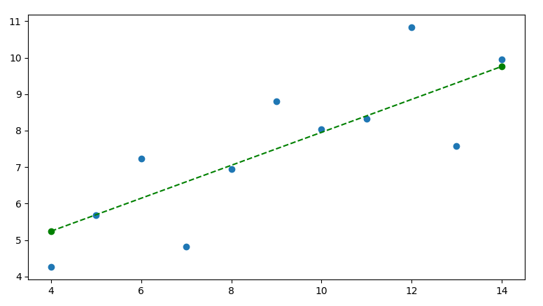
def plotLinearRegression(x, y):
    beginY = predictWithLinearRegression(x, y, min(x))
    endY = predictWithLinearRegression(x, y, endX)

    x1, y1 = [min(x), max(x)], [beginY, endY]
    plt.plot(x1, y1, color="green", linestyle="dashed", marker = 'o')
Invoking this function will add the following line: